While previous work has developed algorithmic approaches to attacking and defending Variational Autoencoders (VAEs), there remains a lack of formalization for what it even means for a VAE to be robust to adversarial attack.

In adversarial settings an agent is trying to alter the behavior of a model towards a specific goal. This could involve, in the case of classification, adding a very small perturbation to an input so as to alter the model’s predicted class. For many deep learning models small changes to data imperceptible to the human eye can drastically change a model’s output.

Here we briefly review the inherent adversarial robustness of VAEs.

Variational Autoencoders

Before introducing VAEs, we quickly describe variational Bayesian methods, a set of inference methods which underpin the training of VAEs.

• Variational Bayesian methods are a family of techniques for performing inference on intractable integrals, such as calculating the posterior over a set of unobserved latent variables \(\mathbf{z}\) given data \(\mathbf{x}\).

• The posterior distribution over this set of unobserved variables is approximated by a variational distribution \(q​\), \(p(\mathbf{z} \mid \mathbf{x}) \approx q(\mathbf{z})​\), where \(q​\) is chosen to a simpler distribution than ​\(p​\).

• It can be shown that minimising the \(\mathrm{KL}\) divergence between \(q\) and \(p\) is equivalent to maximising the evidence lower bound (ELBO) of the data [2], \(\log p(\mathbf{x}) \geq \log p(\mathbf{x}) - \mathrm{KL}(q\|p) = \mathcal{L}(\mathbf{x}) = \mathbb{E}_{q(\mathbf{z})}[\log p(\mathbf{x},\mathbf{z})] - \mathbb{E}_{q(\mathbf{z})}[\log q(\mathbf{z})]\).

• In the context of VAEs, amortised inference refers to the fact that the parameters of the distributions \(p​\) and \(q​\) are data-dependent, meaning they vary per-datapoint \(\mathbf{x}​\). This amortisation allows for variational inference to scale to very large datasets.

VAEs, and models they have inspired, are deep neural networks that can perform variational inference for high dimensional data and large datasets. They introduce a joint distribution over data \(\mathbf{x}\) (in data-space \(\mathcal{X}\)) and a set of latent variables \(\mathbf{z}\) (in latent-space \(\mathcal{Z}\)), \(p_\theta(\mathbf{x},\mathbf{z})=p_\theta(\mathbf{x}\mid\mathbf{z})p(\mathbf{z})\) where \(p_\theta(\mathbf{x}\mid\mathbf{z})\) is a distribution that matches the properties of the data.

The parameters of the likelihood \(p_\theta(\mathbf{x}\mid\mathbf{z})\) are encoded by neural networks which take in samples of \(\mathbf{z}\). A common choice of prior for the space \(\mathcal{Z}\) is the unit normal Gaussian, \(p(\mathbf{z})=\mathcal{N}(0,\mathcal{I})\). As exact inference for these models is intractable, one performs amortised stochastic variational inference by introducing another inference network for the latent variables, \(q_\phi(\mathbf{z}\mid\mathbf{x})\), which often encodes the parameters of another Gaussian, \(\mathcal{N}(\mu_\phi(\mathbf{x}),\Sigma_\phi(\mathbf{x}))​\) [2].

In the case of VAEs, given the factorisation of \(p​\) specified above and given the amortisation of inference we can write,

\[\mathcal{L}(\mathbf{x})=\mathbb{E}_{q_\phi(\mathbf{z}\mid\mathbf{x})} \left[\log p_\theta(\mathbf{x}\mid\mathbf{z})\right] - \mathrm{KL}(q_\phi(\mathbf{z}\mid\mathbf{x}) \| p(\mathbf{z}))\]

\(q_\phi\) is typically referred to as the encoder network and \(p_\theta\) is referred to as the decoder network. To propagate gradients during gradient descent through the distributions and into the networks that parameterise them, we use the reparameterisation trick.

For Gaussian variational posteriors for example we draw samples from \(q_\phi(\mathbf{z}\mid\mathbf{x})\) as

\[\mu_\phi(\mathbf{x}) + \mathbf{\epsilon}\sigma_\phi(\mathbf{x}), \mathbf{\epsilon} \sim \mathcal{N}(\mathbf{0}, \mathbf{I})​\]

where \(\mu_\phi(\mathbf{x})\) and \(\sigma_\phi(\mathbf{x})\) are the mean and standard deviation parameterised by the encoder. We coin this layer the ‘stochastic’ layer of the VAE. We approximate the likelihood using samples from this stochastic layer. Draws from \(p_\theta(\mathbf{x}\mid\mathbf{z})\) are termed ‘reconstructions’ of the original data \(\mathbf{x}\) in the VAE literature. We can also use these samples to approximate the \(\mathrm{KL}​\) divergence, but it has a tractable form in the case of Gaussian distributions.

The Adversarial Robustness of VAEs

Generally, VAEs and VAE inspired models, such as Variational Information Bottleneck have been found to be more resilient to input perturbations (and also more targeted attacks) than their deterministic counterparts. Nevertheless these models are still susceptible to attacks from adversaries.

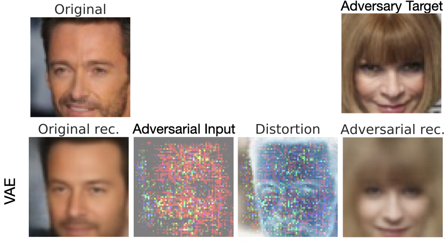
Currently proposed attacks for Variational Autoencoder (VAEs) aim to produce reconstructions close to a chosen target image by applying small distortions to the input of a VAE [1]. The adversary optimizes this perturbation to minimize some measure of distance between the reconstruction and the target image or the distance between the embedding of the distorted image and the embedding of the target image.

In the image below we give an example of adversarial attacks on the CelebA dataset. We start with the image of Hugh Jackman in the top left and have an adversary that tries to produce reconstructions that look like Anna Wintour as per the top right. This is done by applying a distortion (third column) to the original image to produce an adversarial input (second column). We can see that the adversarial reconstruction for the VAE looks substantially like Wintour, indicating a successful attack. This figure is taken from my paper.

A probabilistic metric of robustness

Deep learning models can be brittle. Some of the most sophisticated deep learning classifiers can be broken by simply adding small pertubations to their inputs. Here, perturbations that would not fool a human break neural network predictions. A model’s weakness to such perturbations is called its sensitivity. For classifiers, we can straightforwardly define an associated sensitivity margin, it is the radius of the largest metric ball centered on an input \(\mathbf{x}\) for which a classifier’s original prediction holds for all possible perturbations within that ball.

Defining such a margin for VAEs is conceptually more difficult as, in general, the reconstructions are continuous rather than discrete. To put it another way, there is no step-change in VAE reconstructions that is akin to a change of a predicted class in classifiers; any perturbation in the input space will result in a change in the VAE output. To complicate matters further, a VAE’s latent space is stochastic, the same input can result in different reconstructions.

My recent paper makes inroads towards defining a sensitivity margin, which we call \(r​\)-robustness, for probabilistic models.

r-robustness: A model, \(f\), operating on a point \(\mathbf{x}\), that outputs a continuous random variable is \(r\)-robust for \(r \in \mathbb{R}^+\), to a perturbation \(\mathbf{\delta}\) and for an arbitrary norm \(\|\cdot\|\) if and only if \(p(\|f(\mathbf{x} + \mathbf{\delta}) - f(\mathbf{x})\| \leq r) > p(\|f(\mathbf{x} + \mathbf{\delta}) - f(\mathbf{x})\| > r).​\)

We will assume from now on that the norm is taken to be the 2-norm \(\|\cdot\|_2​\), such that \(r​\)-robustness determines a bound for which changes in the output \(f(\mathbf{x})​\) induced by the perturbation \(\mathbf{\delta}​\) are more likely to fall within the hyper-sphere of radius \(r​\), than not. As \(r​\) decreases, the criterion for model robustness becomes stricter.

Because this criterion is applicable to probabilistic models with continuous output spaces, it is directly relevant for ascertaining robustness in VAEs. By considering the smallest \(r\) for which the criterion holds, we can think of it as a metric that provides a probabilistic measure of the extent to which outputs are altered given a corrupted input, the smaller the value of \(r\) for which we can confirm \(r\)-robustness, the more robust the model.

A Robustness Margin for VAEs

We want to define a margin in a VAE’s input space for which it is robust to perturbations of a given input. Perturbations that fall within this margin should not break our criterion for robustness.

Formally, we want a margin in \(\mathcal{X}\), \(R^r_{\mathcal{X}}(\mathbf{x})\), for which any distorted input \(\mathbf{x}+\delta_x\), where \(\|\mathbf{\delta}_x\|_2 < R^r_{\mathcal{X}}(\mathbf{x})\) is the perturbation, satisfies \(r\)-robustness when reconstructed.

r-robustness for VAEs

However, to consider the robustness of VAEs, we must not only take into account the perturbation \(\mathbf{\delta}_x\), but also the stochasticity of encoder. We can think of the decoder as taking in noisy inputs because of this stochasticity.Naturally, this noise can itself potentially cause issues in the robustness of VAE, if the level of noise is too high, we will not achieve reliable reconstructions even without perturbing the original inputs.As such, before even considering perturbations, we first need to adapt our \(r​\)-robustness framework to deal with this stochasticity.

We illustrate \(r\)-robustness in a VAE visually in the image below. White dots represent possible reconstructions, with the diversity originating from the encoder stochasticity.For \(r\)-robustness to hold, the probability of our reconstruction falling within the red area—a hypersphere of radius \(r\) centered on \(g_{\theta}(\mathbf{\mu}_\phi(\mathbf{x}))\) —needs to be greater than or equal to the probability of falling outside. We denote \(g_{\theta}(\mathbf{z})\) as the deterministic mapping induced by the VAE’s decoder network and \(\mathbf{\mu}_\phi(\mathbf{x})\) as the mean embedding of the encoder, we can define \(g_{\theta}(\mathbf{\mu}_\phi(\mathbf{x}))\) to be the ‘maximum likelihood’ reconstruction, noting that this is a deterministic function.

Using this definition we can begin to charaterise the margin of robustness of a VAE.

A margin of robustness for VAEs

Given that we have established conditions for \(r\)-robustness in that take into account latent space sampling, we can now return to our original objective, which was to determine a margin in the data-space \(\mathcal{X}\) for which a VAE is robust to perturbations on its input. Recall that this implicitly means that we want to define a bound for robustness given two sources of perturbations, the stochasticity of the encoder, and a hypothetical input perturbation \(\mathbf{\delta}_x\).

We illustrate this margin \(R^r_{\mathcal{X}}(\mathbf{x})\), defined in the input space \(\mathcal{X}\), in the image below. Red represents represents the subspace where the model is \(r\)-robust for all perturbed input \(\mathbf{x} + \mathbf{\delta}_x\) falling in this region, that is all \(\mathbf{\delta}_x : \lVert \mathbf{\delta}_x \rVert_2 \le R^r_{\mathcal{X}}(\mathbf{x})\). Conversely blue regions illustrate regions where perturbed inputs break the \(r\)-robustness criterion.

This theorising is all well and good, but can it be used to predict the robustness of models ? Are models with larger margins \(R^r_{\mathcal{X}}(\mathbf{x})​\) more robust to adversarial attack ?

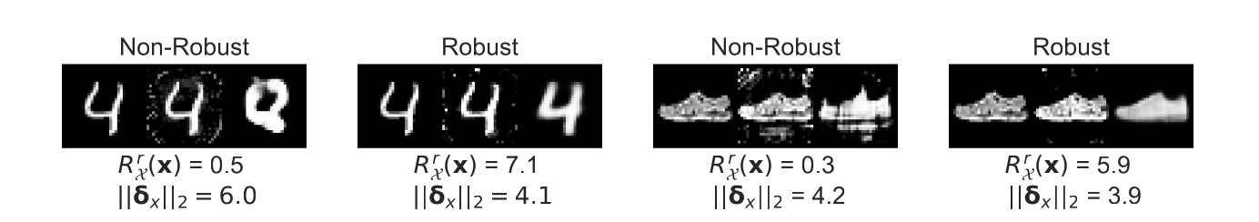
In the image below for instance each subfigure shows from left to right: the original input, a perturbed input made by an adversarial attack, and the reconstruction of the perturbed input. We show results for VAEs that are robust (\(R^r_{\mathcal{X}}(\mathbf{x})\ge\| \delta_x\rVert_2\)) and non-robust (\(R^r_{\mathcal{X}}(\mathbf{x})<\| \delta_x\rVert_2\)) for a given point \(\mathbf{x}\) and adversarially selected perturbation \(\delta_x\). It is clear that the robust VAE reconstructions are visually closer to the original input.

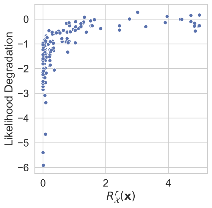
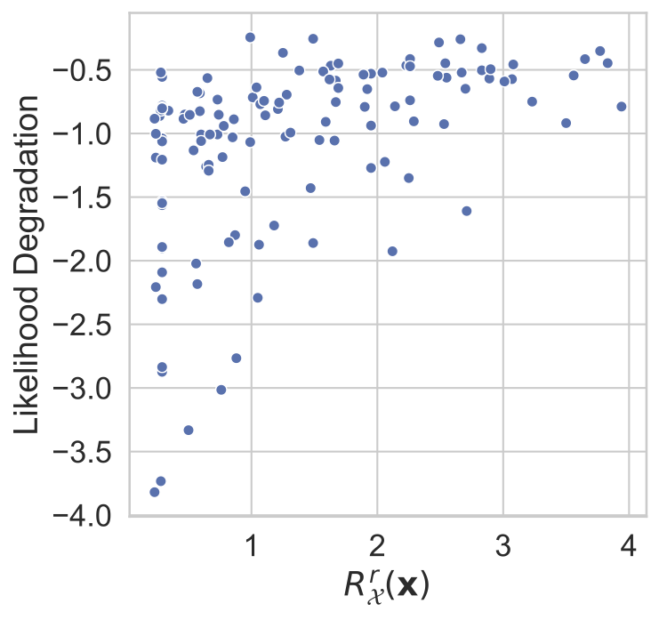
We can quantify this achieved robustness numerically, and we do so by measuring \(R^r_{\mathcal{X}}(\mathbf{x})\) for a range of models and datapoints and subsequently measure the likelihood degradation engendered by adversarial attacks. More precisely, we measure the likelihood of the original point \(\mathbf{x}\) and quantify the degradation in model performance as the relative log likelihood degradation (\(\mid(\log p(\mathbf{x} \mid \mathbf{z}^*) - \log p(\mathbf{x} \mid \mathbf{z})) \mid /\log p(\mathbf{x} \mid \mathbf{z})\)), where \(\mathbf{z}\) is the embedding of \(\mathbf{x}\) and \(\mathbf{z}^*\) is the embedding of \(\mathbf{x} + \delta_x\). \(\delta_x\) is generated using maximum damage attacks. In these attacks an adversary maximizes, with respect to some perturbation \(\delta_x​\), the distance between the VAE reconstruction and the original datapoint \(\mathbf{x}​\). We attack the encoder mean and variance:

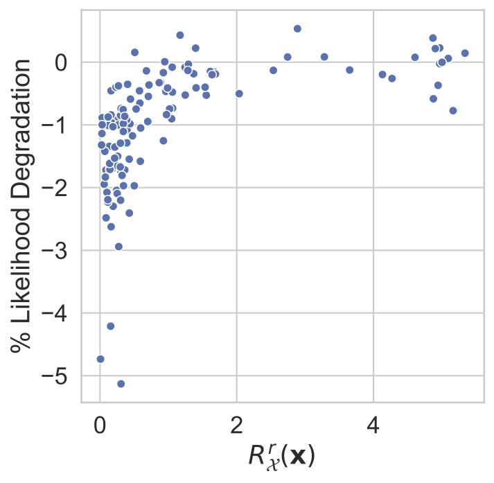
\[\mathbf{\delta}_x^* =\mathrm{argmax}_{\mathbf{\delta}_x}\big(\|g_{\theta}(\mathbf{\mu}_\phi(\mathbf{x} + \mathbf{\delta}_x)+ \mathbf{\eta}\sigma_\phi(\mathbf{x} + \mathbf{\delta}_x)) - g_{\theta}(\mathbf{\mu}_\phi(\mathbf{x}))\|_2\big). ​\]

In the images below it is clear that that as \(R^r_{\mathcal{X}}(\mathbf{x})\) increases the degradation in likelihood engendered by these attacks lessens, indicating less damaging attacks. Larger ‘margins’ of robustness correspond to more robust models.

MNIST	fashion-MNIST	CIFAR10

In our work, we assume that the perturbations to the input only affect the encoder mean, and not the encoder variance, which we find surprisingly to be a faithful approximation to what happens in most adversarial settings. Adversaries do the most damage by attacking the encoder mean, and not by attacking the encoder variance.

Recall that a perturbation in \(\mathcal{X}\), \(\mathbf{\delta}_x\), induces a perturbation in \(\mathcal{Z}\), \(\mathbf{\delta}_z\). To determine the margins for robustness in \(\mathcal{X}\), we first apply the Neyman-Pearson lemma, assuming a ‘worst-case’ decoder. This decoder has subspaces in \(\mathcal{Z}\), where it is is either robust or non-robust, that are divided by a boundary that is normal to both the induced perturbation \(\mathbf{\delta}_z\) and to the dimension of minimal variance in \(\mathcal{Z}\), \(\min_i \mathbf{\sigma}_\phi(\mathbf{x})_i\). We then determine the minimum perturbation norm in \(\mathcal{X}\) which induces a perturbation in \(\mathcal{Z}\) that crosses this boundary.

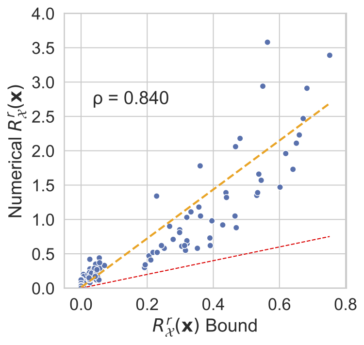
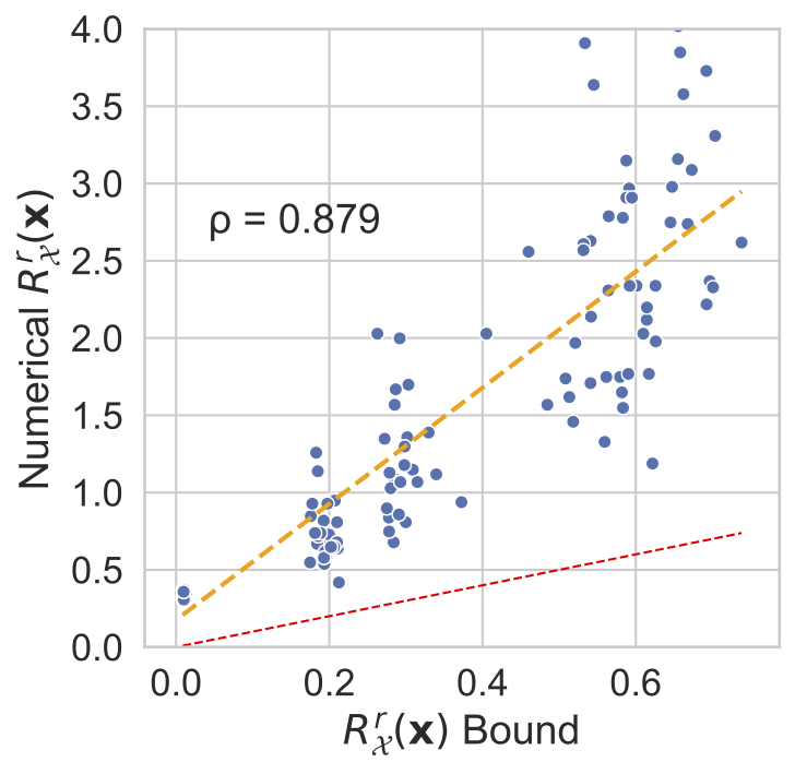
\[R^r_\mathcal{X}(\mathbf{x}) \geq \frac{(\min_i \mathbf{\sigma}_\phi(\mathbf{x})_i)\Phi^{-1}(p(\|\Delta(\mathbf{x})\|_2 \leq r))}{\|\mathbf{J}^{\mu}_{\phi}(\mathbf{x})\|_F } + \mathcal{O} (\mathbf \varepsilon)\]

where \(\mathcal{O} (\varepsilon)​\) represents higher order dominated terms that disappear in the limit of small perturbations, \(\Phi^{-1}​\) is the inverse CDF of the unit normal Gaussian, \(\mathbf{J}^{\mu}_{\phi}(\mathbf{x})_{i,j}=\partial \mathbf{\mu}_\phi(\mathbf{x})_{i} / \partial \mathbf{x}_j​\) , \(\|\cdot\|_F​\) is the Frobenius norm, \(p(\|\Delta(\mathbf{x})\|_2 \leq r)​\) is the probability that \(r​\)-robustness holds before the input is perturbed.

In the figure below we plot numerically estimated margins of robustness against our bound, ignoring higher order terms encapsulated in \(\mathcal{O} (\varepsilon)\). For all three datasets we show our derived bound is a valid lower bound for the true margin of robustness, and is a relatively tight bound.

MNIST	fashion-MNIST	CIFAR10

Note that this bound includes two terms that might contribute to the robustness. The encoder variance plays a prominent role and is a parameter that is easy to control. The encoder Jacobian is also present, but we found that controlling such values directly can be difficult. Nevertheless, we find in my recent paper that \(\beta\)-VAEs [3], which upweight the KL term of the VAE ELBO, induce a regularisation that increases both the encoder variance and penalises large encoder Jacobians. We find that these models are more robust than vanilla VAEs, suggesting that regularising a VAE’s latent space, by acting on the KL, is a viable strategy for inducing robust models.

References

[1] Kos, J., Fischer, I., & Song, D. (2018b). Adversarial Examples for Generative Models. In IEEE Security and Privacy Workshops 2018.

[2] Diederik P. Kingma and Max Welling. Auto-encoding variational bayes, In ICLR 2014

[3] Higgins, I., Matthey, L., Pal, A., Burgess, C., Glorot,X., Botvinick, M., Mohamed, S., & Lerchner, A.(2017a) .β-VAE: Learning Basic Visual Concepts with a Constrained Variational Framework.

[4] Kumar, A. & Poole, B. (2020). On Implicit Regularization in β-VAEs.