My recent Neurips paper, written with my friends and colleagues at the University of Oxford, studies the often used and yet poorly understood method of adding Gaussian noise to data and neural network activations.

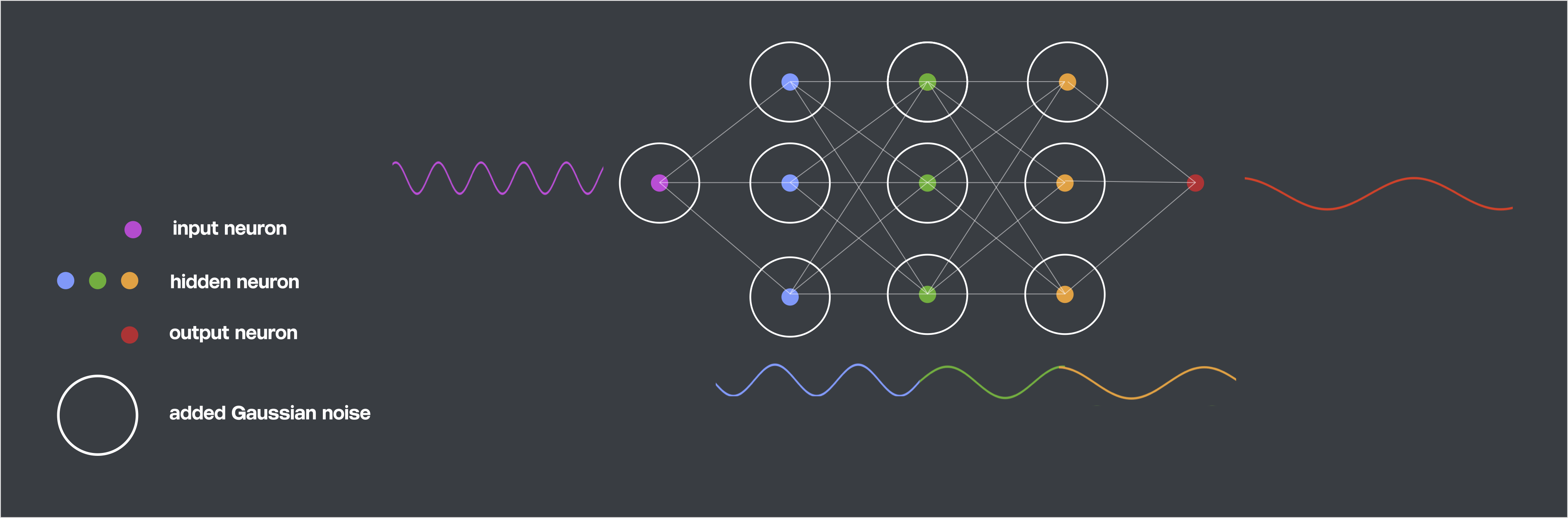
These Gaussian noise injections (GNIs) have an effect in the Fourier domain, which we illustrate in the image below. Each coloured dot represents a neuron’s activations. We add GNIs, represented as circles, to each layer’s activations bar the output layer. GNIs induce a network for which each layer learns a progressively lower frequency function, represented as a sinusoid matching in colour to its corresponding layer.

Gaussian Noise Injections

Consider an feed-forward neural network with \(M\) parameters divided into \(L\) layers: \(\mathbf{\theta} = \{\mathbf{W}_1,...,\mathbf{W}_L\}\), \(\mathbf{\theta} \in \mathbb{R}^M\), and a non-linearity \(\phi\) at each layer. We obtain the activations \(\mathbf{h} = \{\mathbf{h}_0, ... , \mathbf{h}_{L} \}\), where \(\mathbf{h}_{0}=\mathbf{x}\) is the input data before any noise is injected. For a network consisting of dense layers we have that:

\[\mathbf{h}_{k}(\mathbf{x})= \phi(\mathbf{W}_k \mathbf{h}_{k-1}(\mathbf{x}))\]

What happens to these activations when we inject noise? First, let \(\mathbf{\epsilon}\) be the set of noise injections at each layer: \(\mathbf{\epsilon} = \{\mathbf{\epsilon}_0, ... , \mathbf{\epsilon}_{L-1} \}\). When performing a noise injection procedure, the value of the next layer’s activations depends on the noised value of the previous layer. We denote the intermediate, soon-to-be-noised value of an activation as \(\hat{\mathbf{h}}_{k}\) and the subsequently noised value as \(\tilde{\mathbf{h}}_{k}\):

\[\hat{\mathbf{h}}_{k}(\mathbf{x})= \phi\left(\mathbf{W}_{k}\tilde{\mathbf{h}}_{k-1}(\mathbf{x})\right)\,\] \[\tilde{\mathbf{h}}_{k}(\mathbf{x}) = \hat{\mathbf{h}}_{k}(\mathbf{x}) \circ \mathbf{\epsilon}_{k}\,\]

where \(\circ\) is some element-wise operation.

We can, for example, add or multiply Gaussian noise to each hidden layer unit. In the additive case, we obtain:

\[\tilde{\mathbf{h}}_k(\mathbf{x}) = \hat{\mathbf{h}}_k(\mathbf{x}) + \mathbf{\epsilon}_k, \qquad \mathbf{\epsilon}_k \sim \mathcal{N}(0,\sigma_k^2\mathbf{I}).\]

We can express the effect of the Gaussian noise injection on the cost function \(\mathcal{L}\) as an added term \(\Delta\mathcal{L}\), which is dependent on the noise additions \(\mathbf{\epsilon}\) on the previous hidden layer activations. \begin{equation} \tilde{\mathcal{L}}(\mathcal{B};\mathbf{\theta}, \mathbf{\epsilon}) = \mathcal{L}(\mathcal{B}; \mathbf{\theta}) + \Delta\mathcal{L}(\mathcal{B};\mathbf{\theta},\mathbf{\epsilon}_{L}) \end{equation}

Explicit Regularisation of Gaussian Noise Injections

To understand the regularisation induced by GNIs, we want to study the regularisation that these injections induce consistently from batch to batch. To do so, we want to remove the stochastic component of the GNI regularisation and extract a regulariser that is of consistent sign. This consistency of sign is important. Regularisers that change sign batch-to-batch do not give a consistent objective to optimise, making them unfit as regularisers [1].

As such, we study the explicit regularisation these injections induce by way of the expected regulariser \(\mathbb{E}_{\mathbf{\epsilon} \sim p(\mathbf{\epsilon})} \left[ \Delta\mathcal{L}(\cdot) \right]\). Our work demonstrates that this expected regulariser contains a term \(R\) which is the main contributor of the effect of GNIs.

\[R(\mathcal{B}; \mathbf{\theta}) = \mathbb{E}_{(\mathbf{x},\mathbf{y}) \sim \mathcal{B}} \left[\frac{1}{2}\sum_{k=0}^{L-1}\left[\sigma_k^2\mathrm{Tr}\left(\mathbf{J}^T_{k}(\mathbf{x}) \mathbf{H}_{L}(\mathbf{x}, \mathbf{y})\mathbf{J}_{k}(\mathbf{x})\right)\right] \right].\]

Where \(\mathcal{B}\) is a mini-batch process, \((\mathbf{x}, \mathbf{y})\) is a data-label pair and for For compactness of notation, we denote each layer’s Jacobian as \(\mathbf{J}_k \in \mathbb{R}^{d_L \times d_k}\) and the Hessian of the loss with respect to the final layer as \(\mathbf{H}_L \in \mathbb{R}^{d_L \times d_L}\)). Each entry of \(\mathbf{J}_{k}\) is a partial derivative of \(f^k_{\theta,i}(\cdot)​\), the function from layer \(k\) to the \(i^{\mathrm{th}}\) network output, \(i = 1 ... d_L\).

\[\mathbf{J}_{k}(\mathbf{x}) = \begin{bmatrix} \frac{f^k_{\theta,1}}{\partial h_{k,1}} & \frac{f^k_{\theta,1}}{\partial h_{k,2}} & \dots \\ \vdots & \ddots & \\ \frac{f^k_{\theta,d_L}}{\partial h_{k,1}} & & \frac{f^k_{\theta,d_L}}{\partial h_{k,d_k}} \end{bmatrix}\] \[\mathbf{H}_{L}(\mathbf{x}, \mathbf{y}) = \begin{bmatrix} \frac{\partial^2 \mathcal{L}}{\partial h^2_{L,1}} & \frac{\partial^2 \mathcal{L}}{\partial h_{L,1}\partial h_{L,2}} & \dots \\ \vdots & \ddots & \\ \frac{\partial^2 \mathcal{L}}{\partial h_{L,d_L}\partial h_{L,1}} & & \frac{\partial^2 \mathcal{L}}{\partial h^2_{L,d_L}} \end{bmatrix} ​\]

Explicit Regularisation as Fourier Domain Penalisation

By way of Sobolev spaces we show that the above regulariser corresponds to a penalisation in the Fourier domain. When the batch size increases towards the size of the full dataset we can write the regulariser, in the regression setting, as:

\[R(\mathcal{B}; \mathbf{\theta}) = \frac{1}{2}\sum_{k=0}^{L-1} \sigma_k^2 \sum_{i} \int_{\mathbb{R}^{d_k}} \sum^{d_k}_{j=1} \Bigr|\mathcal{G}^k_i(\mathbf{\omega},j)\overline{ \mathcal{G}^k_i(\mathbf{\omega},j) * \mathcal{P}(\mathbf{\omega})}\Bigr| d\mathbf{\omega} ​\]

here \(\mathbf{h}_0 =\mathbf{x}\), \(i\) indexes over output neurons, and \(\mathcal{G}^k_i(\mathbf{\omega}, j) = \mathbf{\omega}_j \mathcal{F}^k_i(\mathbf{\omega})\), where \(\mathcal{F}^k_i\) is the Fourier transform of the function \(f^k_{\theta,i}(\cdot)\). \(\mathcal{P}\) is the Fourier transform or the `characteristic function’ of the data density function.

This term can look pretty overwhelming but the key takeaway here is that the terms \(\mathcal{G}^k_i(\mathbf{\omega}, j)\) become large in magnitude when functions have high-frequency components. This implies that GNIs penalise neural networks that learn functions with high-frequency components.

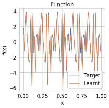
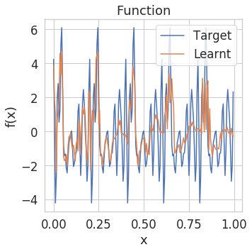
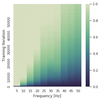
To illustrate what this entails visually, check out the functions learnt by neural networks trained with and without GNIs below. We train neural networks to regress mixtures of sinusoids and plot both the function learnt by the networks and the Fourier transform (FT) of this learnt function as training progresses.

Function no GNIs	Function GNIs

FT no GNIs	FT GNIs

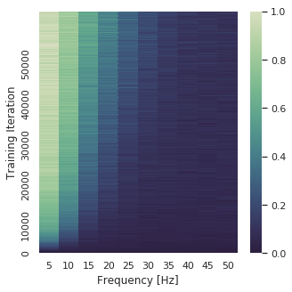It is pretty apparent that the models trained with learn a lower frequency function that is less likely to overfit.

Its also interesting to note that there is a recursive structure to the penalisation induced by \(R(\cdot)\). Consider the layer-to-layer functions which map from a layer \(k-1\) to \(k\), \(\mathbf{h}_{k}(\mathbf{h}_{k-1}(\mathbf{x}))\). \(\|D \mathbf{h}_{k}(\mathbf{h}_{k-1}(\mathbf{x}))\|_2^2\) is penalised \(k\) times in \(R(\cdot)\) as this derivative appears in \(\mathbf{J}_0, \mathbf{J}_1 \dots \mathbf{J}_{k-1}\) due to the chain rule. As such, when training with GNIs, we can expect the norm of \(\|D \mathbf{h}_{k}(\mathbf{h}_{k-1}(\mathbf{x}))\|_2^2\) to decrease as the layer index \(k\) increases (i.e the closer we are to the network output). This norm measure the layer-layer frequency learnt by each \(\mathbf{h}_k\). You can read the paper for the full details of this connection.

Basically larger values of this norm are indicative of layer-layer functions with higher frequency content, and conversely smaller values of this norm are indicative of layer-layer functions with lower frequency content. In networks with \(\mathrm{ReLU}\) activations \(D \mathbf{h}_{k}(\mathbf{h}_{k-1}(\mathbf{x})) = \tilde{\mathbf{W}}_k​\).\(\tilde{\mathbf{W}}_k\) is obtained from the original weight matrix \(\mathbf{W}_k\) by setting its \(i^{\mathrm{th}}​\) column to zero whenever the neuron \(i​\) of the \((k)^{\mathrm{th}}\) layer is inactive.

We plot these norms for each layer in a \(\mathrm{ReLU}\) network. The plot to the left corresponds to the networks trained without GNIs, the plot to the right is for networks trained with GNIs.

no GNIs	GNIs

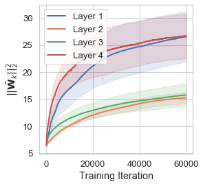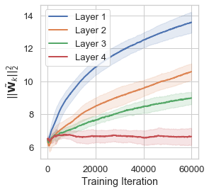For GNI models, deeper layers learn smaller \(\|\tilde{\mathbf{W}}_k\|_2^2\), with the first hidden layer having the largest norm, the second layer having the second largest values and so on so forth. This striation and ordering is notably absent in the models trained without GNIs. This effectively demonstrates that this Fourier domain penalisation disproportionately affects layers nearest to the network output, inducing a network that learns a lower frequency function at each successive layer. ``

References

[1] Aleksandar Botev, Hippolyt Ritter, and David Barber. Practical Gauss-Newton optimisation for deeplearning. In ICML, 2017.